Confidence interval Facts for Kids

In statistics, a confidence interval, abbreviated as CI, is a special interval for estimating a certain parameter, such as the population mean. With this method, a whole interval of acceptable values for the parameter is given instead of a single value—together with a likelihood that the real (unknown) value of the parameter will be in the interval. Thus, if we're not sure of the exact number of vehicles that crossed a bridge, we can say 400 plus or minus 10 instead of just saying 400.

The confidence interval is based on the observations from a sample, and hence differs from sample to sample. The likelihood that the parameter will be in the interval is called the confidence level, and the end points of the confidence interval are referred to as confidence limits.

Very often, this is given as a percentage (for example, the 95% confidence interval). The confidence interval is always given together with the confidence level. For a given estimation procedure in a given situation, the higher the confidence level, the wider the confidence interval will be.

The calculation of a confidence interval generally requires assumptions about the nature of the estimation process, since it is primarily a parametric method. One common assumption is that the distribution of the population from which the sample came is normal. As such, confidence intervals as discussed below are not robust statistics, though changes can be made to add robustness.

Practical example
Related pages
Images for kids
See also

Practical example

A factory assembly line fills margarine cups to a desired 250g +/- 5g

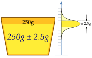
A machine fills cups with margarine. It is adjusted so that the content of the cups is 250g of margarine. As the machine cannot fill every cup with exactly 250g, the content added to individual cups shows some variation, and is considered a random variable X.

This variation is assumed to be normally distributed around the desired average of 250g, with a standard deviation of 2.5g. To determine if the machine is adequately calibrated, a sample of n = 25 cups of margarine is chosen at random, and the cups are weighed. The weights of margarine are X₁, ..., X₂₅, a random sample from X.

To get an impression of the expectation μ, an estimate is needed. The appropriate estimator is the sample mean:

\hat \mu=\bar X = \frac{1}{n}\sum_{i=1}^n X_i.

The sample shows actual weights x₁, ...,x₂₅, with mean:

\bar x=\frac {1}{25} \sum_{i=1}^{25} x_i = 250.2\,\text{grams}.

If we take another sample of 25 cups, we could easily expect to find values like 250.4 or 251.1 grams. A sample mean value of 280 grams, however, would be extremely rare if the mean content of the cups is in fact close to 250g.

There is a whole interval around the observed value 250.2 of the sample mean within which, if the whole population mean actually takes a value in this range, the observed data would not be considered particularly unusual. Such an interval is called a confidence interval for the parameter μ.

To calculate such an interval, the endpoints of the interval have to be calculated from the sample, so they are statistics, functions of the sample X₁, ..., X₂₅, and hence are random variables themselves.

In our case, we may determine the endpoints by considering that the sample mean X from a normally distributed sample is also normally distributed, with the same expectation μ, but with standard error σ/√n = 0.5 (grams). By standardizing, we get a random variable

Z = \frac {\bar X-\mu}{\sigma/\sqrt{n}} =\frac {\bar X-\mu}{0.5}

which depends on the parameter μ to be estimated, but with a standard normal distribution independent of the parameter μ. Hence it is possible to find numbers −z and z, independent of μ, where Z lies in between with probability 1 − α, a measure of how confident we want to be. We take 1 - α = 0.95. So we have:

P(-z\le Z\le z) = 1-\alpha = 0.95. \,

The number z follows from the cumulative distribution function:

\begin{align} \Phi(z) & = P(Z \le z) = 1 - \tfrac{\alpha}2 = 0.975,\\[6pt] z & = \Phi^{-1}(\Phi(z)) = \Phi^{-1}(0.975) = 1.96, \end{align}

and we get:

\begin{align} 0.95 & = 1-\alpha=P(-z \le Z \le z)=P \left(-1.96 \le \frac {\bar X-\mu}{\sigma/\sqrt{n}} \le 1.96 \right) \\[6pt] & = P \left( \bar X - 1.96 \frac{\sigma}{\sqrt{n}} \le \mu \le \bar X + 1.96 \frac{\sigma}{\sqrt{n}}\right) \\[6pt] & = P\left(\bar X - 1.96 \times 0.5 \le \mu \le \bar X + 1.96 \times 0.5\right) \\[6pt] & = P \left( \bar X - 0.98 \le \mu \le \bar X + 0.98 \right). \end{align}

This might be interpreted as: with probability 0.95, we will find a confidence interval in which we will meet the parameter μ between the stochastic endpoints

\bar X - 0{.}98 \,

and

\bar X + 0.98. \,

This does not mean that there is 0.95 probability of meeting the parameter μ in the calculated interval. Every time the measurements are repeated, there will be another value for the mean X of the sample. In 95% of the cases, μ will be between the endpoints calculated from this mean, but in 5% of the cases, it will not be. The actual confidence interval is calculated by entering the measured weights in the formula. Our 0.95 confidence interval becomes:

(\bar x - 0.98;\bar x + 0.98) = (250.2 - 0.98; 250.2 + 0.98) = (249.22; 251.18).\,

The vertical line segments represent 50 realisations of a confidence interval for μ.

As the desired value 250 of μ is within the resulted confidence interval, there is no reason to believe the machine is wrongly calibrated.

The calculated interval has fixed endpoints, where μ might be in between (or not). Thus this event has probability either 0 or 1. We cannot say: "with probability (1 − α), the parameter μ lies in the confidence interval." We only know that by repetition in 100(1 − α) % of the cases, μ will be in the calculated interval. In 100α % of the cases, however, it does not. And unfortunately we do not know in which of the cases this happens. That is why we say: "with confidence level 100(1 − α) %, μ lies in the confidence interval."

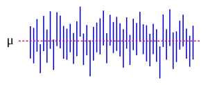
The figure on the right shows 50 realisations of a confidence interval for a given population mean μ. If we randomly choose one realisation, the probability that it contains the parameter is 95%. However, it is also possible that we may have unluckily picked the wrong one as well.

Images for kids

In this bar chart, the top ends of the brown bars indicate observed means and the red line segments ("error bars") represent the confidence intervals around them. Although the error bars are shown as symmetric around the means, that is not always the case. In most graphs, the error bars do not represent confidence intervals (e.g., they often represent standard errors or standard deviations)

Confidence interval facts for kids

Contents

Practical example

Related pages

Images for kids

See also