Normal distribution Facts for Kids

Quick facts for kids
Normal
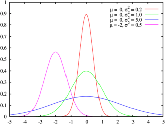
Probability density function The green line is the standard normal distribution
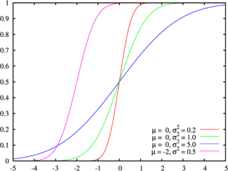
Cumulative distribution function Colors match the image above
Parameters	$\mu$ location (real) $\sigma^2>0$ squared scale (real)
Support	$x \in\mathbb{R}\!$
Probability density function (pdf)	$\frac1{\sigma\sqrt{2\pi}}\; \exp\left(-\frac{\left(x-\mu\right)^2}{2\sigma^2} \right) \!$
Cumulative distribution function (cdf)	$\frac12 \left(1 + \mathrm{erf}\,\frac{x-\mu}{\sigma\sqrt2}\right) \!$
Mean	$\mu$
Median	$\mu$
Mode	$\mu$
Variance	$\sigma^2$
Skewness	0
Excess kurtosis	0
Entropy	$\ln\left(\sigma\sqrt{2\,\pi\,e}\right)\!$
Moment-generating function (mgf)	$M_X(t)= \exp\left(\mu\,t+\frac{\sigma^2 t^2}{2}\right)$
Characteristic function	$\chi_X(t)=\exp\left(\mu\,i\,t-\frac{\sigma^2 t^2}{2}\right)$

The normal distribution is a probability distribution. It is also called Gaussian distribution because it was first discovered by Carl Friedrich Gauss. The normal distribution is a continuous probability distribution that is very important in many fields of science.

Normal distributions are a family of distributions of the same general form. These distributions differ in their location and scale parameters: the mean ("average") of the distribution defines its location, and the standard deviation ("variability") defines the scale. These two parameters are represented by the symbols $\mu$ and $\sigma$ , respectively.

The standard normal distribution (also known as the Z distribution) is the normal distribution with a mean of zero and a standard deviation of one (the green curves in the plots to the right). It is often called the bell curve, because the graph of its probability density looks like a bell.

Many values follow a normal distribution. This is because of the central limit theorem, which says that if an event is the sum of identical but random events, it will be normally distributed. Some examples include:

Height
Test scores
Measurement errors
Light intensity (so-called Gaussian beams, as in laser light)
Intelligence is probably normally distributed. There is a problem with accurately defining or measuring it, though.
Insurance companies use normal distributions to model certain average cases.

Student's t-distribution

Images for kids

As the number of discrete events increases, the function begins to resemble a normal distribution
a: Probability density of a function \cos x^2 of a normal variable x with \mu=-2 and \sigma=3. b: Probability density of a function x^y of two normal variables x and y, where \mu_x=1, \mu_y=2, \sigma_x = 0.1, \sigma_y = 0.2, and \rho_{xy} = 0.8. c: Heat map of the joint probability density of two functions of two correlated normal variables x and y, where \mu_x = -2, \mu_y=5, \sigma_x^2 = 10, \sigma_y^2 = 20, and \rho_{xy} = 0.495. d: Probability density of a function \sum_{i=1}^4 \vert x_i \vert of 4 iid standard normal variables. These are computed by the numerical method of ray-tracing.
The ground state of a quantum harmonic oscillator has the Gaussian distribution.
The bean machine, a device invented by Francis Galton, can be called the first generator of normal random variables. This machine consists of a vertical board with interleaved rows of pins. Small balls are dropped from the top and then bounce randomly left or right as they hit the pins. The balls are collected into bins at the bottom and settle down into a pattern resembling the Gaussian curve.
Carl Friedrich Gauss discovered the normal distribution in 1809 as a way to rationalize the method of least squares.
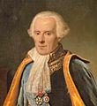
Pierre-Simon Laplace proved the central limit theorem in 1810, consolidating the importance of the normal distribution in statistics.

Normal distribution facts for kids

Related pages

Images for kids

See also