Linear subspace facts for kids

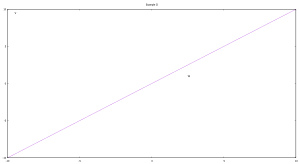
One-dimensional subspaces in the two-dimensional vector space over the finite field F₅. The origin (0, 0), marked with green circles, belongs to any of six 1-subspaces, while each of 24 remaining points belongs to exactly one; a property which holds for 1-subspaces over any field and in all dimensions. All F₅² (i.e. a 5 × 5 square) is pictured four times for a better visualization

In mathematics, and more specifically in linear algebra, a linear subspace or vector subspace is a vector space that is a subset of some larger vector space. A linear subspace is usually simply called a subspace when the context serves to distinguish it from other types of subspaces.

Definition

If V is a vector space over a field K and if W is a subset of V, then W is a linear subspace of V if under the operations of V, W is a vector space over K. Equivalently, a nonempty subset W is a subspace of V if, whenever $w 1, w 2$ are elements of W and $α, β$ are elements of K, it follows that $αw 1 + βw 2$ is in W.

As a corollary, all vector spaces are equipped with at least two (possibly different) linear subspaces: the zero vector space consisting of the zero vector alone and the entire vector space itself. These are called the trivial subspaces of the vector space.

Examples

Example I

In the vector space V = R³ (the real coordinate space over the field R of real numbers), take W to be the set of all vectors in V whose last component is 0. Then W is a subspace of V.

Proof:

Given u and v in W, then they can be expressed as u = (u₁, u₂, 0) and v = (v₁, v₂, 0). Then u + v = (u₁+v₁, u₂+v₂, 0+0) = (u₁+v₁, u₂+v₂, 0). Thus, u + v is an element of W, too.
Given u in W and a scalar c in R, if u = (u₁, u₂, 0) again, then cu = (cu₁, cu₂, c0) = (cu₁, cu₂,0). Thus, cu is an element of W too.

Example II

Let the field be R again, but now let the vector space V be the Cartesian plane R². Take W to be the set of points (x, y) of R² such that x = y. Then W is a subspace of R².

Example II Illustrated

Proof:

Let p = (p₁, p₂) and q = (q₁, q₂) be elements of W, that is, points in the plane such that p₁ = p₂ and q₁ = q₂. Then p + q = (p₁+q₁, p₂+q₂); since p₁ = p₂ and q₁ = q₂, then p₁ + q₁ = p₂ + q₂, so p + q is an element of W.
Let p = (p₁, p₂) be an element of W, that is, a point in the plane such that p₁ = p₂, and let c be a scalar in R. Then cp = (cp₁, cp₂); since p₁ = p₂, then cp₁ = cp₂, so cp is an element of W.

In general, any subset of the real coordinate space Rⁿ that is defined by a system of homogeneous linear equations will yield a subspace. (The equation in example I was z = 0, and the equation in example II was x = y.)

Example III

Again take the field to be R, but now let the vector space V be the set R^R of all functions from R to R. Let C(R) be the subset consisting of continuous functions. Then C(R) is a subspace of R^R.

Proof:

We know from calculus that 0 ∈ C(R) ⊂ R^R.
We know from calculus that the sum of continuous functions is continuous.
Again, we know from calculus that the product of a continuous function and a number is continuous.

Example IV

Keep the same field and vector space as before, but now consider the set Diff(R) of all differentiable functions. The same sort of argument as before shows that this is a subspace too.

Examples that extend these themes are common in functional analysis.

Properties of subspaces

From the definition of vector spaces, it follows that subspaces are nonempty, and are closed under sums and under scalar multiples. Equivalently, subspaces can be characterized by the property of being closed under linear combinations. That is, a nonempty set W is a subspace if and only if every linear combination of finitely many elements of W also belongs to W. The equivalent definition states that it is also equivalent to consider linear combinations of two elements at a time.

In a topological vector space X, a subspace W need not be topologically closed, but a finite-dimensional subspace is always closed. The same is true for subspaces of finite codimension (i.e., subspaces determined by a finite number of continuous linear functionals).

Descriptions

Descriptions of subspaces include the solution set to a homogeneous system of linear equations, the subset of Euclidean space described by a system of homogeneous linear parametric equations, the span of a collection of vectors, and the null space, column space, and row space of a matrix. Geometrically (especially over the field of real numbers and its subfields), a subspace is a flat in an n-space that passes through the origin.

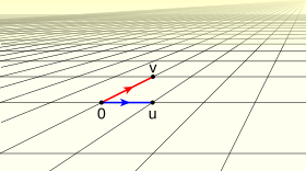
A natural description of a 1-subspace is the scalar multiplication of one non-zero vector v to all possible scalar values. 1-subspaces specified by two vectors are equal if and only if one vector can be obtained from another with scalar multiplication:

\exist c\in K: \mathbf{v}' = c\mathbf{v}\text{ (or }\mathbf{v} = \frac{1}{c}\mathbf{v}'\text{)}

This idea is generalized for higher dimensions with linear span, but criteria for equality of k-spaces specified by sets of k vectors are not so simple.

A dual description is provided with linear functionals (usually implemented as linear equations). One non-zero linear functional F specifies its kernel subspace F = 0 of codimension 1. Subspaces of codimension 1 specified by two linear functionals are equal, if and only if one functional can be obtained from another with scalar multiplication (in the dual space):

\exist c\in K: \mathbf{F}' = c\mathbf{F}\text{ (or }\mathbf{F} = \frac{1}{c}\mathbf{F}'\text{)}

It is generalized for higher codimensions with a system of equations. The following two subsections will present this latter description in details, and the remaining four subsections further describe the idea of linear span.

Systems of linear equations

The solution set to any homogeneous system of linear equations with n variables is a subspace in the coordinate space Kⁿ: ${\displaystyle \left\{ \left[\!\! \begin{array}{c} x_1 \\ x_2 \\ \vdots \\ x_n \end{array} \!\!\right] \in K^n : \begin{alignat}{6} a_{11} x_1 &&\; + \;&& a_{12} x_2 &&\; + \cdots + \;&& a_{1n} x_n &&\; = 0& \\ a_{21} x_1 &&\; + \;&& a_{22} x_2 &&\; + \cdots + \;&& a_{2n} x_n &&\; = 0& \\ && && && && && \vdots\quad& \\ a_{m1} x_1 &&\; + \;&& a_{m2} x_2 &&\; + \cdots + \;&& a_{mn} x_n &&\; = 0& \end{alignat} \right\}. }$

For example, the set of all vectors $(x, y, z)$ (over real or rational numbers) satisfying the equations $x + 3y + 2z = 0 \quad\text{and}\quad 2x - 4y + 5z = 0$ is a one-dimensional subspace. More generally, that is to say that given a set of n independent functions, the dimension of the subspace in K^k will be the dimension of the null set of A, the composite matrix of the n functions.

Null space of a matrix

In a finite-dimensional space, a homogeneous system of linear equations can be written as a single matrix equation:

A\mathbf{x} = \mathbf{0}.

The set of solutions to this equation is known as the null space of the matrix. For example, the subspace described above is the null space of the matrix

A = \begin{bmatrix} 1 & 3 & 2 \\ 2 & -4 & 5 \end{bmatrix} .

Every subspace of Kⁿ can be described as the null space of some matrix (see Linear subspace § Notes below for more).

Linear parametric equations

The subset of Kⁿ described by a system of homogeneous linear parametric equations is a subspace:

\left\{ \left[\!\! \begin{array}{c} x_1 \\ x_2 \\ \vdots \\ x_n \end{array} \!\!\right] \in K^n : \begin{alignat}{7} x_1 &&\; = \;&& a_{11} t_1 &&\; + \;&& a_{12} t_2 &&\; + \cdots + \;&& a_{1m} t_m & \\ x_2 &&\; = \;&& a_{21} t_1 &&\; + \;&& a_{22} t_2 &&\; + \cdots + \;&& a_{2m} t_m & \\ && \vdots\;\; && && && && && & \\ x_n &&\; = \;&& a_{n1} t_1 &&\; + \;&& a_{n2} t_2 &&\; + \cdots + \;&& a_{nm} t_m & \\ \end{alignat} \text{ for some } t_1,\ldots,t_m\in K \right\}.

For example, the set of all vectors (x, y, z) parameterized by the equations

x = 2t_1 + 3t_2,\;\;\;\;y = 5t_1 - 4t_2,\;\;\;\;\text{and}\;\;\;\;z = -t_1 + 2t_2

is a two-dimensional subspace of K³, if K is a number field (such as real or rational numbers).

Span of vectors

In linear algebra, the system of parametric equations can be written as a single vector equation:

\begin{bmatrix} x \\ y \\ z \end{bmatrix} \;=\; t_1 \!\begin{bmatrix} 2 \\ 5 \\ -1 \end{bmatrix} + t_2 \!\begin{bmatrix} 3 \\ -4 \\ 2 \end{bmatrix}.

The expression on the right is called a linear combination of the vectors (2, 5, −1) and (3, −4, 2). These two vectors are said to span the resulting subspace.

In general, a linear combination of vectors v₁, v₂, ... , v_k is any vector of the form

t_1 \mathbf{v}_1 + \cdots + t_k \mathbf{v}_k.

The set of all possible linear combinations is called the span:

\text{Span} \{ \mathbf{v}_1, \ldots, \mathbf{v}_k \} = \left\{ t_1 \mathbf{v}_1 + \cdots + t_k \mathbf{v}_k : t_1,\ldots,t_k\in K \right\} .

If the vectors v₁, ... , v_k have n components, then their span is a subspace of Kⁿ. Geometrically, the span is the flat through the origin in n-dimensional space determined by the points v₁, ... , v_k.

Example

The xz-plane in R³ can be parameterized by the equations

x = t_1, \;\;\; y = 0, \;\;\; z = t_2.

As a subspace, the xz-plane is spanned by the vectors (1, 0, 0) and (0, 0, 1). Every vector in the xz-plane can be written as a linear combination of these two:

(t_1, 0, t_2) = t_1(1,0,0) + t_2(0,0,1)\text{.}

Geometrically, this corresponds to the fact that every point on the xz-plane can be reached from the origin by first moving some distance in the direction of (1, 0, 0) and then moving some distance in the direction of (0, 0, 1).

Column space and row space

A system of linear parametric equations in a finite-dimensional space can also be written as a single matrix equation:

\mathbf{x} = A\mathbf{t}\;\;\;\;\text{where}\;\;\;\;A = \left[ \begin{alignat}{2} 2 && 3 & \\ 5 && \;\;-4 & \\ -1 && 2 & \end{alignat} \,\right]\text{.}

In this case, the subspace consists of all possible values of the vector x. In linear algebra, this subspace is known as the column space (or image) of the matrix A. It is precisely the subspace of Kⁿ spanned by the column vectors of A.

The row space of a matrix is the subspace spanned by its row vectors. The row space is interesting because it is the orthogonal complement of the null space (see below).

Independence, basis, and dimension

The vectors u and v are a basis for this two-dimensional subspace of R³.

In general, a subspace of Kⁿ determined by k parameters (or spanned by k vectors) has dimension k. However, there are exceptions to this rule. For example, the subspace of K³ spanned by the three vectors (1, 0, 0), (0, 0, 1), and (2, 0, 3) is just the xz-plane, with each point on the plane described by infinitely many different values of t₁, t₂, t₃.

In general, vectors v₁, ... , v_k are called linearly independent if

t_1 \mathbf{v}_1 + \cdots + t_k \mathbf{v}_k \;\ne\; u_1 \mathbf{v}_1 + \cdots + u_k \mathbf{v}_k

for (t₁, t₂, ... , t_k) ≠ (u₁, u₂, ... , u_k). If v₁, ..., v_k are linearly independent, then the coordinates t₁, ..., t_k for a vector in the span are uniquely determined.

A basis for a subspace S is a set of linearly independent vectors whose span is S. The number of elements in a basis is always equal to the geometric dimension of the subspace. Any spanning set for a subspace can be changed into a basis by removing redundant vectors (see § Algorithms below for more).

Example

Let S be the subspace of R⁴ defined by the equations

x_1 = 2 x_2\;\;\;\;\text{and}\;\;\;\;x_3 = 5x_4.

Then the vectors (2, 1, 0, 0) and (0, 0, 5, 1) are a basis for S. In particular, every vector that satisfies the above equations can be written uniquely as a linear combination of the two basis vectors:

(2t_1, t_1, 5t_2, t_2) = t_1(2, 1, 0, 0) + t_2(0, 0, 5, 1).

The subspace S is two-dimensional. Geometrically, it is the plane in R⁴ passing through the points (0, 0, 0, 0), (2, 1, 0, 0), and (0, 0, 5, 1).

Operations and relations on subspaces

Inclusion

The set-theoretical inclusion binary relation specifies a partial order on the set of all subspaces (of any dimension).

A subspace cannot lie in any subspace of lesser dimension. If dim U = k, a finite number, and U ⊂ W, then dim W = k if and only if U = W.

Intersection

In R³, the intersection of two distinct two-dimensional subspaces is one-dimensional

Given subspaces U and W of a vector space V, then their intersection U ∩ W := {v ∈ V : v is an element of both U and W} is also a subspace of V.

Proof:

Let v and w be elements of U ∩ W. Then v and w belong to both U and W. Because U is a subspace, then v + w belongs to U. Similarly, since W is a subspace, then v + w belongs to W. Thus, v + w belongs to U ∩ W.
Let v belong to U ∩ W, and let c be a scalar. Then v belongs to both U and W. Since U and W are subspaces, cv belongs to both U and W.
Since U and W are vector spaces, then 0 belongs to both sets. Thus, 0 belongs to U ∩ W.

For every vector space V, the set {0} and V itself are subspaces of V.

Sum

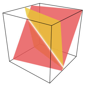
If U and W are subspaces, their sum is the subspace $U + W = \left\{ \mathbf{u} + \mathbf{w} \colon \mathbf{u}\in U, \mathbf{w}\in W \right\}.$

For example, the sum of two lines is the plane that contains them both. The dimension of the sum satisfies the inequality $\max(\dim U,\dim W) \leq \dim(U + W) \leq \dim(U) + \dim(W).$

Here, the minimum only occurs if one subspace is contained in the other, while the maximum is the most general case. The dimension of the intersection and the sum are related by the following equation: $\dim(U+W) = \dim(U) + \dim(W) - \dim(U \cap W).$

A set of subspaces is independent when the only intersection between any pair of subspaces is the trivial subspace. The direct sum is the sum of independent subspaces, written as $U \oplus W$ . An equivalent restatement is that a direct sum is a subspace sum under the condition that every subspace contributes to the span of the sum.

The dimension of a direct sum $U \oplus W$ is the same as the sum of subspaces, but may be shortened because the dimension of the trivial subspace is zero.

$\dim (U \oplus W) = \dim (U) + \dim (W)$

Lattice of subspaces

The operations intersection and sum make the set of all subspaces a bounded modular lattice, where the {0} subspace, the least element, is an identity element of the sum operation, and the identical subspace V, the greatest element, is an identity element of the intersection operation.

Orthogonal complements

If $V$ is an inner product space and $N$ is a subset of $V$ , then the orthogonal complement of $N$ , denoted $N^{\perp}$ , is again a subspace. If $V$ is finite-dimensional and $N$ is a subspace, then the dimensions of $N$ and $N^{\perp}$ satisfy the complementary relationship $\dim (N) + \dim (N^{\perp}) = \dim (V)$ . Moreover, no vector is orthogonal to itself, so $N \cap N^\perp = \{ 0 \}$ and $V$ is the direct sum of $N$ and $N^{\perp}$ . Applying orthogonal complements twice returns the original subspace: $(N^{\perp})^{\perp} = N$ for every subspace $N$ .

This operation, understood as negation ( $\neg$ ), makes the lattice of subspaces a (possibly infinite) orthocomplemented lattice (although not a distributive lattice).

In spaces with other bilinear forms, some but not all of these results still hold. In pseudo-Euclidean spaces and symplectic vector spaces, for example, orthogonal complements exist. However, these spaces may have null vectors that are orthogonal to themselves, and consequently there exist subspaces $N$ such that $N \cap N^{\perp} \ne \{ 0 \}$ . As a result, this operation does not turn the lattice of subspaces into a Boolean algebra (nor a Heyting algebra).

Algorithms

Most algorithms for dealing with subspaces involve row reduction. This is the process of applying elementary row operations to a matrix, until it reaches either row echelon form or reduced row echelon form. Row reduction has the following important properties:

The reduced matrix has the same null space as the original.
Row reduction does not change the span of the row vectors, i.e. the reduced matrix has the same row space as the original.
Row reduction does not affect the linear dependence of the column vectors.

Basis for a row space

Input An m × n matrix A.

Output A basis for the row space of A.

Use elementary row operations to put A into row echelon form.
The nonzero rows of the echelon form are a basis for the row space of A.

See the article on row space for an example.

If we instead put the matrix A into reduced row echelon form, then the resulting basis for the row space is uniquely determined. This provides an algorithm for checking whether two row spaces are equal and, by extension, whether two subspaces of Kⁿ are equal.

Subspace membership

Input A basis {b₁, b₂, ..., b_k} for a subspace S of Kⁿ, and a vector v with n components.

Output Determines whether v is an element of S

Create a (k + 1) × n matrix A whose rows are the vectors b₁, ... , b_k and v.
Use elementary row operations to put A into row echelon form.
If the echelon form has a row of zeroes, then the vectors {b₁, ..., b_k, v} are linearly dependent, and therefore v ∈ S.

Basis for a column space

Input An m × n matrix A

Output A basis for the column space of A

Use elementary row operations to put A into row echelon form.
Determine which columns of the echelon form have pivots. The corresponding columns of the original matrix are a basis for the column space.

See the article on column space for an example.

This produces a basis for the column space that is a subset of the original column vectors. It works because the columns with pivots are a basis for the column space of the echelon form, and row reduction does not change the linear dependence relationships between the columns.

Coordinates for a vector

Input A basis {b₁, b₂, ..., b_k} for a subspace S of Kⁿ, and a vector v ∈ S

Output Numbers t₁, t₂, ..., t_k such that v = t₁b₁ + ··· + t_kb_k

Create an augmented matrix A whose columns are b₁,...,b_k , with the last column being v.
Use elementary row operations to put A into reduced row echelon form.
Express the final column of the reduced echelon form as a linear combination of the first k columns. The coefficients used are the desired numbers t₁, t₂, ..., t_k. (These should be precisely the first k entries in the final column of the reduced echelon form.)

If the final column of the reduced row echelon form contains a pivot, then the input vector v does not lie in S.

Basis for a null space

Input An m × n matrix A.

Output A basis for the null space of A

Use elementary row operations to put A in reduced row echelon form.
Using the reduced row echelon form, determine which of the variables x₁, x₂, ..., x_n are free. Write equations for the dependent variables in terms of the free variables.
For each free variable x_i, choose a vector in the null space for which x_i = 1 and the remaining free variables are zero. The resulting collection of vectors is a basis for the null space of A.

See the article on null space for an example.

Basis for the sum and intersection of two subspaces

Given two subspaces $U$ and $W$ of $V$ , a basis of the sum $U + W$ and the intersection $U \cap W$ can be calculated using the Zassenhaus algorithm.

Equations for a subspace

Input A basis {b₁, b₂, ..., b_k} for a subspace S of Kⁿ

Output An (n − k) × n matrix whose null space is S.

Create a matrix A whose rows are b₁, b₂, ..., b_k.
Use elementary row operations to put A into reduced row echelon form.
Let c₁, c₂, ..., c_n be the columns of the reduced row echelon form. For each column without a pivot, write an equation expressing the column as a linear combination of the columns with pivots.
This results in a homogeneous system of n − k linear equations involving the variables c₁,...,c_n. The (n − k) × n matrix corresponding to this system is the desired matrix with nullspace S.

Example: If the reduced row echelon form of A is

\left[ \begin{alignat}{6} 1 && 0 && -3 && 0 && 2 && 0 \\ 0 && 1 && 5 && 0 && -1 && 4 \\ 0 && 0 && 0 && 1 && 7 && -9 \\ 0 && \;\;\;\;\;0 && \;\;\;\;\;0 && \;\;\;\;\;0 && \;\;\;\;\;0 && \;\;\;\;\;0 \end{alignat} \,\right]

then the column vectors c₁, ..., c₆ satisfy the equations

\begin{alignat}{1} \mathbf{c}_3 &= -3\mathbf{c}_1 + 5\mathbf{c}_2 \\ \mathbf{c}_5 &= 2\mathbf{c}_1 - \mathbf{c}_2 + 7\mathbf{c}_4 \\ \mathbf{c}_6 &= 4\mathbf{c}_2 - 9\mathbf{c}_4 \end{alignat}

It follows that the row vectors of A satisfy the equations

\begin{alignat}{1} x_3 &= -3x_1 + 5x_2 \\ x_5 &= 2x_1 - x_2 + 7x_4 \\ x_6 &= 4x_2 - 9x_4. \end{alignat}

In particular, the row vectors of A are a basis for the null space of the corresponding matrix.

Linear subspace facts for kids

Contents

Definition

Examples

Example I

Example II

Example III

Example IV

Properties of subspaces

Descriptions

Systems of linear equations

Null space of a matrix

Linear parametric equations

Span of vectors

Column space and row space

Independence, basis, and dimension

Operations and relations on subspaces

Inclusion

Intersection

Sum

Lattice of subspaces

Orthogonal complements

Algorithms

Basis for a row space

Subspace membership

Basis for a column space

Coordinates for a vector

Basis for a null space

Basis for the sum and intersection of two subspaces

Equations for a subspace

See also